VLOOKUP To The Left With INDEX MATCH

Anyone who has used Excel for a while uses VLOOKUP.


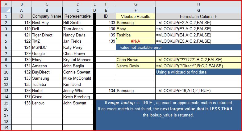
In the below example I use VLOOKUP to pull back the location of an employee based on the user Id.

However VLOOKUP cannot look to the left. What if I knew the State but did not know the employee?                   

If I wanted to use VLOOKUP, I would need to rearrange the columns putting the Employee Name in Column D.                                

That’s because you cannot use negative numbers in a VLOOKUP formula to return columns to the left).                               

                               

To get around the limitation you can use a combination of INDEX and MATCH to lookup up data to the left.                         

                               

=INDEX($A$2:$C$6, MATCH(E2,$C$2:$C$6, FALSE),2)

I placed the above formula in cellF2 and search on the Location, can return the employee name.                              

                               

So what is this formula doing??? Let’s break it down.                     

                               

In English, INDEX goes to the data range and returns you the value in the intersection of the row number and the column number.                             

                               

                               

                               

                               

                               

I can replace the row lookup in the above formula with the MATCH function.                     

                               

The MATCH function will tell the Index function which row to look at.                    

Four our purpose, MATCH tells Excel to search the data range and find the relative row number where you find a match.                               

                               

=MATCH(E3,$C$2:$C$6, FALSE) will return the number 3 since Iowa is the 3rd row in the array (column  C) data                 

                               

Putting the two functions together gives you the super user ability to look to the left in Excel.                   

                               

So how do I select the column of data to return?                             

                               

Remember our range is three columns, A B and C.  If you want to return the data in Column A, select 1, Column B use 2 and column C put 3.                

                               

If I wanted to return the Id number I can put a 1 at the end of the formula                          

                               

=INDEX($A$2:$C$6, MATCH(E2,$C$2:$C$6, FALSE),1)                      

                               

In fact you can use the INDEX MATCH combination to completely replace VLOOKUP as it will allow you to look left or right of you lookup value.    


Now that you know the secret, how will you use INDEX MATCH?        

VLOOKUP

+

Vlookup is one of the most useful functions available in Excel.

There are times that you will need to pull in data from different sections or tabs of a workbook (or even different workbooks).

Let’s say that you want to identify the Company Name for each of our Items in our sample workbook. VLookup will search for a value you provide in the left most column of a range of data and return the value in the same row based on an index number that represents the column where the data resides that you want to return. Confused???

Simply put, VLOOKUP allows you to search for an item and pull back related information to that item.

Take a look at our sample data. Columns A B and C has data about vendors. For my example I have also entered in the ID of some vendors in column E. I want to use VLOOKUP to return the Company name for each ID in column E.  I have entered in my VLOOKUP formula in column F. To see the formula, I have also typed the exact formula that I used in column F in Column G.

You will notice that in cell F5 I have a “value not available error”. This is because in cell E13 I have the value 134. That value is not included in my lookup range. (This can be corrected by using the IFERROR(VLOOKUP combination.)

If you compare one of my calculations in my sample workbook, you can see how each component works.

=VLOOKUP(E2,A:C,2,FALSE)

VLookup( value, table_array, index_number, not_exact_match )

Value: The value I want to search for (133).                                                                    

table_array: Is a selection of data that is at least two columns wide that is sorted in ascending order by the first column in the array (Columns A B and C).                                                                  

index_number: The column # in table_array where the data you want returned is stored in. Regardless of where you start your table_array, the first column is number 1. (2 – Return Column B)                         

Not_exact_match: True or False option. Enter False to return an exact match. Enter TRUE to find an approximate match. If no exact match is found, True will look for the next largest value that is less than value 

(False – find an exact match).

Wildcards

If range_lookup is FALSE and lookup_value is text, you can use the wildcard characters - (?) and asterisk (*).

A question mark matches any single character (as shown in cell F8 in my example).

 If you have 6 question marks, then you are trying to return a field with 6 characters in length.

An asterisk matches any sequence of characters.

 If you want to find an actual question mark or asterisk, type a tilde (~) preceding the character.

VLOOKUP also has a cousin called HLOOKUP but that’s a topic for another time.

How have you used VLOOKUP to solve a problem?

Trim Function

One of the more useful functions in Excel is the Trim function.

=TRIM(text)

Trim does exactly what is sounds like, it trims white space from the front and end of text. This is crucial if you are using the text in a lookup.

lets say in cell A1 you have the following text "  this has spaces in the front and back     "
in cell B1 type =TRIM(A1)
the value is converted to "this has spaces in the front and back". The spaces in the front and back of the text are removed. Now you can use this value in a =VLOOKUP function.

COUNTIF to identify patterns in your data

Count If can be used to identify patterns in your data. For instance… It’s quite common to have addresses not broken out neatly. This can often be the case with imported data.

In this example I would like to know how many records of addresses are from North Carolina. However my data is not consistent. The state could be referenced as NC or North Carolina. It could also be misspelled as in cell A6 or joined together as in cell A5.

I can use the =COUNTIF formula with wildcards to give me my answer.

However I just can’t rush into my formula. I need to examine my data to identify the best solution.  If I was to search for North, I would get an incorrect count since there is an instance of the word North in Cell A8 that is not part of the state name North Carolina. Also Cell A3 does not have the word North in it.

If I search for the word Carolina with the below formula I also get an incorrect answer as there is a typo for Carolina in cell A6 (don’t you just hate typos).

=COUNTIF(A3:A8,"*Carolina*") + COUNTIF(A3:A8,"*NC*")

So I hedge my formula to avoid the common typos for my search and use the following formula…

=COUNTIF(A3:A8,"*C*ina*") + COUNTIF(A3:A8,"*NC*")

Basically I want to see if there is any short name reference to North Carolina (NC) or if there is any portion of Carolina in the range.

Now data validation is always key when you are asked to produce hard numbers. However using wildcards can help eliminate bad data from your results. 

How would you have approached the solution to this problem?

Sales Dashboard

Here is an example of a good sales dashboard. All the graphics are based on the data in Columns B C and D.  This is a good example of what can be done with just some basic Excel skills.

How would you improve on this dashboard?

Here is the hyperlink on how to build this dashboard.

http://excelprofessor.blogspot.com/2011/08/best-dashboard.html

Conditional Formatting Font Colors To Indicate Change In Profit

There are times when we want to call attention to key items in data. Perhaps it’s a change in profit or drop in inventory. Keeping the data all in one color can cause someone to overlook the key point of a report.

Fortunately Excel allows us to use Conditional Formatting to resolve this problem. In this example I have the same data displayed two ways. I have highlighted the Profit column in the second version to indicate if the value has gone up, down or remained the same.

By using Conditional Formatting on only the one column of data, I point out the most important part of the report and provide the reader a quick visual way to see how the data is trending (without having to manually compare each value to identify the trend).

To create this report, I start with my first chart then use formulas to reproduce it.

Yes I know that I could just apply the conditional formatting to my original data but that would spoil the cool bling bling technique that I will apply later on in this lesson.

I want to start my conditional formatting on the second row of data as the first row does not have any reference to prior value. I select Cell I3 and then Create a New Conditional Formatting Rule


Home > Conditional Formatting > New Rule > Use a formula to determine which cells for format.

The formula I want to enter is =D2<D3. I want to select the format button and select a blue color for the font. Now whenever the current cell is greater than the previous cell, the font will be blue.

I repeat the process with a red font

but make the formula =D2>D3.

When done, I have two rules….

Next I just copy I3 down to all the other cells in column I for the remaining months.


This image is of the Conditional Formatting Rules Manager after I have copied the formatting into the rest of the other cells.

Now your spreadsheet is Da Bomb…. Or is it???

Try replacing the formula in cell I3 with the following…

=D3 & " " & IF(D2<D3,"▲", IF(D2=D3,"●","▼"))

Now copy it down to the other cells below.

Please, keep your applause down to a minimum……


What this formula does if append the value of D3 with either and up arrow, down arrow or dot.
=D3 & " " & IF(D2<D3,"▲", IF(D2=D3,"●","▼"))

That’s why I could not just apply the conditional formatting to my original data at the beginning of this lesson. I wanted to be able to add the indicators to my value.

Getting the indicators takes a bit of fore thought. When you want to create this formula from scratch, do it in MS Word and you can find the indicator when you insert a symbol. Once you have the formula written, copy it back to Excel.

How about breaking out the indicators into the adjacent column and then you could format the Profit column with an Accounting Number format?

If you can do that, then you could also change the arrows to match the color of the numbers

Lastly my favorite, black text for the numbers with blue and red indicators in the helper column. I have created the boarders so it appears to be in the same cell.


































Break out this technique at the next quarterly review and watch everyone’s face as they try to figure out how you did this.