Gantt chart with conditional formatting - EASY

The other day a manager stopped by my desk and asked me if I could help them with a problem they were having with creating a Gantt chart. He had a manager meeting in 15 minutes and he wanted to put together a Gantt chart for the meeting. Now granted he had worked on it for a few hours before stopping by so it’s not like he waited until the last minute.
Well it was time to break out the mad crazy Excel skills (actually it’s quite easy to do but let’s keep that secret to ourselves).
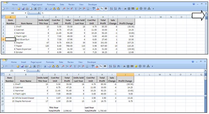
All you need to create a Gantt chart is a few bits of information and two formulas and you can have one that looks like this.


I first created a list of project activities with start and end dates. Then I created a “calendar” with the start date and end date with increments of 7 days. Make sure to format the calendar as short date.
Now, whenever a day falls between start and end day for a corresponding activity, I want to highlight that cell so I first need to identify if the calendar date falls between the start and end date.
=IF(AND(D$3>=$B4, D$3<=$C4),1,"")
That returns a 1 in the cell D4.
I used the $ sign in the formula to lock the calendar date. Next I just copy the formula into all the calendar cells (D4 through AG13).


Now all my cells that meet the criteria have a 1. In the above example I have made the font blue.
Next I use conditional formatting to fill the cell the same blue color whenever the cell value = 1.
Highlight all the cells between D4 through AG13.
Go to Conditional formatting dialog (in 2007, Home tab > Conditional Formatting > New Rule…)


Select Use a formula to determine which cells to format. And enter in the following formula. Then select the format button and choose the fill tab and select the same blue color that you made the numbers.


The last step is to sit back and bask in the glowing compliments of your boss.

Download the example here.

AVERAGEIFS to return an average between dates

I was asked to find the average sales between two date ranges. Well in earlier posts I described how to use SUMIFS and COUNTIFS to get the sum of values between two dates and to count the number of rows between two dates.
Well another cousin of SUMIFS and COUNTIFS is AVERAGIFS.
AVERAGEIFS allows you to get an average of a range of data base on specific criteria(s) (hence the IFS in AVERAGETFS).


In the above example I have a few columns of Data. I want the average total in Column C that have a date range between 1/5/2011 AND 1/20/2011. The formula is in Cell E2 but I show it to you in Cell D2.
=AVERAGEIFS(C:C,B:B,">1/5/2011",B:B,"<1/20/2011")
If I build the formula with the function Argument dialog box, it would look like the following…


Looking at the data sorted by date, I can see that my calculation is correct since the total of the cells highlighted in yellow is 18,000. When I divide that by 4, I get 4,500.


Some notes on the AVERAGEIFS function….
AVERAGEIFS(average_range,criteria_range1,criteria1,criteria_range2,criteria2…)
Average_range is one or more cells to average, including numbers or names, arrays, or references that contain numbers.
Some samples of the AVERAGEIFS criteria are as follows….
45 – no quotes are required for numbers.
“Invoice” – needs quotes around it since it is text.
“>50” – needs quotes around it since it includes the > sign.
D7 – no quotes requires as it references a cell.
If a cell in a criteria range is empty, AVERAGEIFS treats it as a 0 value.
You can use the wildcard characters— the question mark (?) and asterisk (*) — in criteria. A question mark matches any single character, and an asterisk matches any sequence of characters. If you want to find an actual question mark or asterisk, type a tilde (~) before the character.
This formula is not available in Excel 2003 or older.
How have you used AVERAGEIFS to resolve a problem?

New Window – See two tabs at the same time using ALT + W then N

Okay, you have a file with two tabs and would like to be able to see both tabs at the same time.  Sure you could save the spreadsheet and open the saved copy in another window but who has time for that.
Press and hold the ALT and W key at the same time. Release both keys then press the N key.
Ta Da! You now have you one file displayed in two windows. Now you can click on a different tab is each window. Best of all, since it’s still one document, when you make changes on one tab, the change impacts both windows.
Confused???
Basically when you do this you have the same Excel Workbook shown in a vertical fashion.  This lets you view different sections of the same data at the same time.
Need to see three tabs at once? Just do the ALT + W then N again.
You can also select New Window from the View Tab. This does the same as ALT + W then N. Clicking Arrange All will allow you to see the different windows.


The next time the boss and you are working together. Show off and use this trick to ensconce yourself as the Excel expert of your team.

Separating First and Last Names

One of the more common tasks you may come across is breaking out data from inside a cell. I am often asked to separate first and last names that are joined together in one cell. In this example I show a simple way to separate first and last names. I use a series of formulas to accomplish this task, FIND, MID, LEFT, LEN, TRIM and ISERROR.


Last name formula used in Column B
=LEFT(A2,IF(ISERROR(FIND(",",A2,1)),LEN(A2),FIND(",",A2,1)-1))

First name formula used in Column C

=TRIM(IF(ISERROR(FIND(",",A2,1)),A2,MID(A2,FIND(",",A2,1)+1, IF(ISERROR(FIND(" ",A2,FIND(",",A2,1)+2)),LEN(A2), FIND(" ",A2,FIND(",",A2,1)+2))-FIND(",",A2,1))))

How do you accomplish this task?

DATEDIF To Calculate Differences In Dates

One of the less known functions in Excel is =DATEDIF.


You can use the function =DATEDIF to calculate the difference between dates. 


In the below example, I calculate in Cell B3 the difference between the date of June 10, 2011 and Date Born. I then convert the calculation into an easy to read reference.


What ways can you apply this formula?

COUNTIF to identify duplicate data

Excel provides a easy way to eliminate duplicate data. But what if you want to know what data is duplicated.

Well the solution is the function COUNTIF

The COUNTIF function is used to count up the number of cells in a selected range that meet certain criteria.

The syntax for the COUNTIF function is:
=COUNTIF ( Range, Criteria)

Range - the group of cells the function is to search. 

Criteria - determines whether the cell is to be counted or not. This can be a number, expression, cell reference, or text string. 


In this example I have the formula in Column B. I show the formula entered in Column B in Column C.


Using COUNTIF in this manor allows you to identify how many instances of each value in the range of data in Column A. Anything greater then 1 is at least duplicated. In this example there are some triplicate results (indicated by the #3).


How do you identify duplicate data?

Split Screen

If you still need more space you can try to split the window by double clicking in the corner, just above scroll-bar


This will lock the data above the cell where your curser was and allow you to scroll the below data. 


This can be especially helpful when reviewing large amounts of data. 


Zoom

You can change the zoom level to show more cells. You can control the zoom from the View tab of the Ribbon.


The zoom feature can also be access at the bottom right corner of Excel.


Collapse The Ribbon

Double clicking on Ribbon menu tab names will collapse the Ribbon to give you more space. This can be handy if you wish to see a few more rows on the screen but Excel can’t display them due to your screen size and resolution.


Closing Excel

The Office button at the top left hand corner of Excel can be double clicked on to quickly close Excel. This allows you a quick and easy way to close Excel.


If you have made changes to your file, Excel will prompt you to confirm if you wish to save the changes before closing.

Full Screen View

Excel allows you to view the workbook on the entire screen. 


From the View tab of the Ribbon you can select the Full Screen command. 


To return to the normal screen view, press the Esc key on the keyboard.

Navigation

Double clicking the side of a cell will scroll to last cell with data in the row (a blank cell will stop the curser).


You can also double click on the cell top or bottom to scroll up or down the column (a blank cell will stop the curser).


This is a handy way to quickly move around your data but be careful. If you click on the lower right corner of a cell instead of the side or bottom, Excel will auto fill in data.

Go To Using F5

In an earlier post, I mentioned that the last cell in Excel was XFD1048576.

If you needed to scroll from cell A1 to cell XFD1048576, you could use the arrow keys on the keyboard but it will take you some time to get there. Fortunately Excel allows you to jump to a specific cell. Just press the F5 function key on your keyboard.


The Go To dialog box will appear. Just type the cell you want to go to and click the OK button.

If you click on the Special button, the Go To Special dialog box will appear.


Control Commands Using The Keyboard


Key
Description
CTRL+B
Add or remove Bold Formatting.
CTRL+W
Closes the selected workbook.
CTRL+SHIFT+)
Column Unhide within selected columns.
CTRL+'
Copies a formula from the cell above the active cell into the cell.
CTRL+C
Copies selected cells. CTRL+C followed by another CTRL+C shows the Clipboard.
CTRL+ALT+V
Displays the Paste Special dialog box. Available only after you have cut or copied an object, text, or cell contents or contents in another program.
CTRL+SHIFT+$
Currency format with two decimal places. Negative numbers are shown with parentheses.
CTRL+;
Current date.
CTRL+SHIFT+:
Current time.
CTRL+SHIFT+#
Date format with day, month and year.
CTRL+8
Displays / hides the outline symbols.
CTRL+T
Displays the Create Table dialog box.
CTRL+Minus (-)
Displays the Delete dialog box.
CTRL+H
Displays the Find and Replace dialog box (replace tab selected).
CTRL+1
Displays the Format Cells dialog box.
CTRL+SHIFT+Plus (+)
Displays the Insert dialog box.
CTRL+D
Fill Down command copies the contents and format of the topmost cell of a selected range into the cells below.
CTRL+R
Fill Right command copies the contents and format of the left most cell of a selected range into the cells to the right.
CTRL+SHIFT+ ~
General number format.
CTRL+0 or CTRL +9
Hides selected columns / Hides selected Rows.
CTRL+K
Displays the hyperlink dialog box for new hyperlinks or the Edit Hyperlink dialog box for selected existing hyperlinks.
CTRL+A
If the worksheet has data, CTRL+A selects the current region. Pressing CTRL+A a second time selects the current region and any summary rows.
CTRL+V
Inserts the contents of the Clipboard at the insertion point and replaces any selection. Available only after you have cut or copied an object, text, or cell contents.
CTRL+I
Italic formatting applied or removed from text.
CTRL+SHIFT+!
Number format with two decimal places, thousands separator, and minus sign (-) for negative values.
CTRL+SHIFT_
Outline border is remove from selected cells.
CTRL+SHIFT+&
Outline border is applied to the selected cells.
CTRL+SHIFT+%
Percentage format with no decimal places.
CTRL+Y
Repeats the last command or action.
CTRL+SHIFT+(
Row Unhide within selected rows.
CTRL+SHIFT+*
Selects the current region around active cells (all the data encompassed by blank rows and blank columns).
CTRL+SHIFT+@
Time format with the hour and minute, with AM or PM.
CTRL+U
Underlining applying or removing.
CTRL+Z
Undo command to reverse the last command or to delete the last entry typed.


Function Commands Using The Keyboard


Key
Description
F1
Displays the Excel help task pane.

CTRL+F1 Displays / hides the Ribbon.

ALT+F1 Creates a chart of the data in the current range.

ALT+SHIFT+F1 Insert a new worksheet.
F2
Edits the active cell and positions the insertion point at the end of the cell contents.

SHIFT+F2 Add or edit cell comments.

CTRL+F2 Displays the print preview window.
F3
Displays the paste name dialog box.

SHIFT+F3 Display the insert function dialog box.
F4
Repeats the last command or action, if possible.

CTRL+F4 Close the selected workbook.
F5
Displays the go to dialog box.

CTRL+F5 Restore the window size of the selected workbook.
F6
Switches between the worksheet, Ribbon, task pane, and Zoom controls. In a worksheet that has been split (View menu, Manage This Window, Freeze Panes, Split Window command), F6 includes the split panes when switching between panes and the Ribbon area.

SHIFT+F6 Switch between the worksheet, task pane, Ribbon and zoom controls.

CTRL+F6 Switch to the next workbook window when more than one workbook is open.
F7
Check spelling in the active worksheet or selected range.

CTRL+F7 Runs the move command on the workbook window when it is not maximized. Use the arrow keys to move the window, and when finished press ENTER, or ESC to cancel.
F8
Turns extend mode on / off. In extend mode, Extended Selection appears in the status line. The keyboard arrow keys extend the selection.
 F8
cont. 
SHIFT+F8 Enables you to add a nonadjacent cell or range to a selection of cells by using the arrow keys.
CTRL+F8 Performs the size command on the control menu for the workbook when a workbook is not maximized.
ALT+F8 Displays the Macro dialog box to create, run, edit, or delete a macro.
F9
Calculates all worksheets in all open workbooks.

SHIFT+F9 Calculate the active worksheet.

CTRL+ALT+F9 Calculate all worksheets in all open workbooks.

CTRL+ALT+SHIFT+F9 Rechecks dependent formulas and then calculates all cells in all open workbooks, including cells not marked as needing to be calculated.

CTRL+F9 Minimize a workbook window.
F10
Turns key tips on or off.

SHIFT+F10 Display the shortcut menu.

ALT+SHIFT+F10 Displays the menu or message for a smart tag. If more than one smart tag is present, Excel will switch to the next smart tag and display its menu or message.

CTRL+F10 Maximize or restore the workbook window.
F11
Creates a chart of the data in the current range.

SHIFT+F11 Insert a new worksheet.

ALT+F11 Open the visual basic editor for macros.
F12
Display the save as dialog box.