I have been doing this blog for a few months and have steady visitors. Thanks for stopping by.
What changes to the format / layout would make this blog better?
Also what would you like me to write about?
Please take a moment to let me know.
Thanks

Importing Data From Access To Excel
I spend a great deal of time moving data from one application to another. A good example of this is when I need to import data from Access into Excel.
Now I could of course copy my data then paste special CSV format my data from Access to Excel. I do this quite often when my dataset is less than one or two thousand rows. But what if my dataset is quite large (say 500,000 rows)? The clipboard only will hold around 64 thousand rows.
Well Excel allows you to easily import data from Access with just a few steps. Best of all, you can record these steps into a macro for future use (such as a weekly report).
To start you need to make sure the data is in a list with no blank rows or columns within the list. This is easily done with Access as basic datasheets and queries in Access are already formatted this way.
Next from the Data tab, select From Access.


Out of the gate my connection never works. However, since I am only interested in “Reading” data from Access, I click on the Advanced tab and check Read in Access permissions. I also uncheck all other boxes. I find that this one step resolves 99 percent of my connection issues.


Now I could of course copy my data then paste special CSV format my data from Access to Excel. I do this quite often when my dataset is less than one or two thousand rows. But what if my dataset is quite large (say 500,000 rows)? The clipboard only will hold around 64 thousand rows.
Well Excel allows you to easily import data from Access with just a few steps. Best of all, you can record these steps into a macro for future use (such as a weekly report).
To start you need to make sure the data is in a list with no blank rows or columns within the list. This is easily done with Access as basic datasheets and queries in Access are already formatted this way.
Next from the Data tab, select From Access.

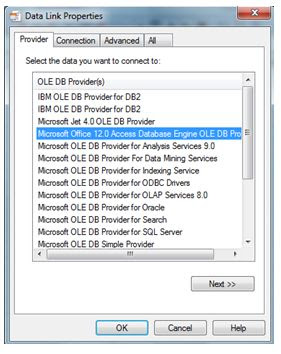
You will be prompted to select the data source (i.e. the Access database with the information you want). I select the drive and folder where my database is and then double click on the database. This opens the Data Link Properties dialog box.
Now this has four tabs (provider, Connection, Advanced and All).

Ensure Microsoft Office 12.0 Access Database Engine is selected on the Provider Tab.
The Connection tab will display your data source (i.e. database name and location). In my example the database is called test.mdb and is located on my C drive.

If you need a user name and PW that is different from the server you are on, you can enter it on this tab. The Connection tab also has a Test Connection button. Click on the button to ensure that Excel can get to the data. If Excel can, you will get a “Test Connection Succeeded” message. If it does not succeed, you will get a “Test connection failed message”. Now depending on how your network security is configured, you may need to tweak a setting or two to make this work. Also if the Access database is protected by a password, you will be prompted to enter it.

I can click back on the Connection tab and test again. This time with my Read Access permissions I am successful.
Once I have a successful test, I click on the OK button at the bottom of the Data Link Properties Dialog Box.
The Select Table Dialog Box will appear. Now this will display all queries and tables that you have the right to use.

Clicking the OK button will cause the Import Data Dialog Box to display. Here you can choose how you want to display the imported data and where you want the data to go in your worksheet.

Clicking the OK button will complete the importing of the Data.
However if you need to have the data refreshed at a given time interval you can select the Properties button. Here you can choose how often the data is updated. There are also options on how to handle the data on the Connections Properties Dialog Box.

So importing data from Access to Excel is not difficult at all. Give it a try the next time someone on your team wants to copy and paste large amounts of data from Access to Excel and “Wow” them with your mad crazy Excel skills.
KPI Dashboard
KPI stands for Key Performance Indicator. KPIs are goals or targets that measure how well a company is doing with achieving its overall operational objectives. KPIs need to be clearly defined in order to provide a quantifiable and measurable indication of progress towards achieving goals.
Since they are defined and measurable, dashboards are an excellent tool for tracking KPIs. Let’s examine how to create a simple, effective KPI dashboard for the ACME Company. Here are the products that the ACME Company sells (primarily to coyote’s).
| Item | Units Sold | Unit Sold Price | Per Unit Profit | Cost To Make Unit | Total Sale $ | Total Cost $ | Total Profit $ |
| Coyote First Aid Kit | 4,050 | 16.89 | 1.79 | 15.10 | 68,404.50 | 61,155.00 | 7,249.50 |
| Blank Signs | 1,046 | 2.45 | 2.23 | 0.22 | 2,562.70 | 230.12 | 2,332.58 |
| Knife and Forks | 1,181 | 1.98 | 1.76 | 0.22 | 2,338.38 | 259.82 | 2,078.56 |
| Road Paint | 2,330 | 1.15 | 0.89 | 0.26 | 2,679.50 | 605.80 | 2,073.70 |
| 500 Lb. Anvil | 2,093 | 1.15 | 0.98 | 0.17 | 2,406.95 | 355.81 | 2,051.14 |
| Hypno Ray gun | 1,859 | 1.23 | 0.99 | 0.23 | 2,286.57 | 427.57 | 1,840.41 |
| Giant Round Boulder | 1,358 | 1.37 | 1.26 | 0.10 | 1,860.46 | 135.80 | 1,711.08 |
| Parachute | 832 | 2.02 | 1.85 | 0.17 | 1,680.64 | 141.44 | 1,539.20 |
| Paint Brushes | 1,815 | 0.97 | 0.70 | 0.26 | 1,760.55 | 471.90 | 1,270.50 |
| Giant Sling Shot | 2,175 | 0.70 | 0.54 | 0.16 | 1,522.50 | 348.00 | 1,174.50 |
| Giant Bow and Arrows | 2,086 | 0.86 | 0.54 | 0.32 | 1,793.96 | 667.52 | 1,126.44 |
| 1000 Lb. Anvil | 878 | 1.38 | 1.27 | 0.10 | 1,211.64 | 87.80 | 1,115.06 |
| Wings | 588 | 1.89 | 1.65 | 0.24 | 1,111.32 | 141.12 | 970.20 |
| Tunnel Paint | 1,670 | 0.87 | 0.56 | 0.31 | 1,452.90 | 517.70 | 935.20 |
| Strap On Helicopter | 868 | 1.25 | 1.01 | 0.24 | 1,085.00 | 208.32 | 876.68 |
| Hole Paint | 1,125 | 1.32 | 0.78 | 0.55 | 1,485.00 | 618.75 | 877.50 |
| Ball Bearings | 1,164 | 0.70 | 0.68 | 0.02 | 814.80 | 23.28 | 791.52 |
| Rocket Launcher | 2,000 | 1.25 | 0.38 | 0.88 | 2,500.00 | 1,760.00 | 760.00 |
| Sign Paint | 1,152 | 0.70 | 0.51 | 0.19 | 806.40 | 218.88 | 587.52 |
| Giant Spring | 722 | 1.07 | 0.80 | 0.27 | 772.54 | 194.94 | 577.60 |
| Aviator Goggles | 1,011 | 0.80 | 0.70 | 0.10 | 808.80 | 101.10 | 707.70 |
| Large Hammer | 2,263 | 0.39 | 0.24 | 0.16 | 882.57 | 362.08 | 543.12 |
| Metal Bird Seed | 1,850 | 0.78 | 0.28 | 0.49 | 1,443.00 | 906.50 | 518.00 |
| Roller Skates | 1,000 | 1.56 | 0.33 | 1.23 | 1,560.00 | 1,230.00 | 330.00 |
| Red Rocket | 1,375 | 1.11 | 0.23 | 0.87 | 1,526.25 | 1,196.25 | 316.25 |
| Helmets | 5 | 1.17 | 1.08 | 0.09 | 5.85 | 0.45 | 5.40 |
Now we need to define our KPIs.
If I look at my data, I have 7 KPIs to start with. I could also add other KPI criteria such as target sale goals, length of time the product sits on the display shelf, etc. but for this example let’s keep it simple and use what we already have in our data.
| KPI 1 | KPI 2 | KPI 3 | KPI 4 | KPI 5 | KPI 6 | KPI 7 |
| Units Sold | Unit Sold Price | Per Unit Profit | Cost To Make Unit | Total Sale $ | Total Cost $ | Total Profit $ |
To start I need to create two tabs in addition to my data tab, Calculations and DASHBOARD.
On the Calculation Tab I want to add two sections, one for Top 5 Values by KPI and the second, Top 5 Product Names by KPI.
Right about now you’re saying to yourself… Now hold on there! How did he do that?
The Top 5 Values by KPI is simple using the LARGE function
LARGE(array,k)
Array is the array or range of data for which you want to determine the k-th largest value.
K is the position (from the largest) in the array or cell range of data to return.
If array is empty, LARGE returns the #NUM! error value.
If k ≤ 0 or if k is greater than the number of data points, LARGE returns the #NUM! error value.
If n is the number of data points in a range, then LARGE(array,1) returns the largest value, and LARGE(array,n) returns the smallest value.
Cell B4 value is =LARGE(Data!B$3:B$28,1)
Cell B5 value is =LARGE(Data!B$3:B$28,2)
As for the Top 5 Product Names by KPI…
Well a while back I showed you have to do a VLookup to the Left using a combination of Index and Match. Don’t recall seeing how it works, insert link here. If I did not want to use Index and Match, I could order my data with ITEM in the last column instead of the first or I could add a helper column to the right that has the same value as the Item column. I could then use VLOOKUP to get my data (but where is the fun in that??? And how would you learn Index Match???).
I use the the Top 5 Values by KPI as my matching value. Here is the first row each KPI column.
=INDEX(Data!$A$3:$B$28,MATCH(B4,Data!$B$3:$B$28,0),1)
=INDEX(Data!$A$3:$C$28,MATCH(C4,Data!$C$3:$C$28,0),1)
=INDEX(Data!$A$3:$D$28,MATCH(D4,Data!$D$3:$D$28,0),1)
=INDEX(Data!$A$3:$E$28,MATCH(E4,Data!$E$3:$E$28,0),1)
=INDEX(Data!$A$3:$F$28,MATCH(F4,Data!$F$3:$F$28,0),1)
=INDEX(Data!$A$3:$G$28,MATCH(G4,Data!$G$3:$G$28,0),1)
=INDEX(Data!$A$3:$H$28,MATCH(H4,Data!$H$3:$H$28,0),1)
For the subsequent rows, I just change the value of the highlighted red cell reference. For example, =INDEX(Data!$A$3:$B$28,MATCH(B4,Data!$B$3:$B$28,0),1) Would become
=INDEX(Data!$A$3:$B$28,MATCH(B5,Data!$B$3:$B$28,0),1)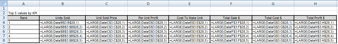
When done, I have the following…
Now I want to create my Dashboard tab.
I format the entire worksheet white background and then add the Top 5 Products by KPI.
I use a simple concatenate to lookup each columns data against the calculations tab. For cell C5 I use the following formula… =CONCATENATE(Calculations!B12," - ",Calculations!B4).

So the top of my KPI dashboard gives the user a quick high level overview of the top products in each KPI (with value) that I am measuring.
Now let’s look at comparing two KPI values.
Back on the Calculation tab I add my KPI Values and assign them the name KPI Values.

I want to use this on my dashboard for KPI comparisons.

I repeat the process in cells B14 and B 15 for my second KPI value. Now when a user clicks on one of these cells, they will be prompted to select a value.

On my calculations tab I add in cell J1 through P1 the following…
| KPI 1 | KPI 2 | KPI 3 | KPI 4 | KPI 5 | KPI 6 | KPI 7 |
I want to return the appropriate values whenever a user enters one of the 7 KPIs in either KPI Value 1 or KPI Value 2.
On the Calculations tab in cells C19 and D 19 I add two Column Headers
| Selected KPI 1 | Selected KPI 2 |
Underneath these Headers I want to return the values for each of the selected KPIs. In this example the user on the Dashboard tab has selected the following two KPIs to compare. To return the value selected, I simply call the cell value
Cell C20 =Dashboard!C12
Cell D 20 =Dashboard!C14
| Selected KPI 1 | Selected KPI 2 |
| Unit Sold Price | Total Profit $ |
Now using an IF OR combination formula I can determine which KPI the user has selected.
For Units Sold I would use the following formula in cell J2 to check of the user has selected Units Sold in either data validation cell.
In cell J2 I use
=IF(OR(Calculations!$C$20 = "Units Sold", Calculations!$D$20 = "Units Sold"),Data!B2,NA())
Column K Units Sold Price formula
In cell K2 I use =IF(OR(Calculations!$C$20 = "Unit Sold Price", Calculations!$D$20 = "Unit Sold Price"),Data!C2,NA())
I then copy this formula down to complete my array ensuring that I change the KPI name and the cell return reference highlighted in red . When done I have dynamic data based on my users selection.
| KPI 1 | KPI 2 | KPI 3 | KPI 4 | KPI 5 | KPI 6 | KPI 7 |
| #N/A | Unit Sold Price | #N/A | #N/A | #N/A | #N/A | Total Profit $ |
| #N/A | 16.89 | #N/A | #N/A | #N/A | #N/A | 7249.5 |
| #N/A | 2.45 | #N/A | #N/A | #N/A | #N/A | 2332.58 |
| #N/A | 1.98 | #N/A | #N/A | #N/A | #N/A | 2078.56 |
| #N/A | 1.15 | #N/A | #N/A | #N/A | #N/A | 2073.7 |
| #N/A | 1.15 | #N/A | #N/A | #N/A | #N/A | 2051.14 |
| #N/A | 1.23 | #N/A | #N/A | #N/A | #N/A | 1840.41 |
| #N/A | 1.37 | #N/A | #N/A | #N/A | #N/A | 1711.08 |
| #N/A | 2.02 | #N/A | #N/A | #N/A | #N/A | 1539.2 |
| #N/A | 0.97 | #N/A | #N/A | #N/A | #N/A | 1270.5 |
| #N/A | 0.7 | #N/A | #N/A | #N/A | #N/A | 1174.5 |
| #N/A | 0.86 | #N/A | #N/A | #N/A | #N/A | 1126.44 |
| #N/A | 1.38 | #N/A | #N/A | #N/A | #N/A | 1115.06 |
| #N/A | 1.89 | #N/A | #N/A | #N/A | #N/A | 970.2 |
| #N/A | 0.87 | #N/A | #N/A | #N/A | #N/A | 935.2 |
| #N/A | 1.25 | #N/A | #N/A | #N/A | #N/A | 876.68 |
| #N/A | 1.32 | #N/A | #N/A | #N/A | #N/A | 877.5 |
| #N/A | 0.7 | #N/A | #N/A | #N/A | #N/A | 791.52 |
| #N/A | 1.25 | #N/A | #N/A | #N/A | #N/A | 760 |
| #N/A | 0.7 | #N/A | #N/A | #N/A | #N/A | 587.52 |
| #N/A | 1.07 | #N/A | #N/A | #N/A | #N/A | 577.6 |
| #N/A | 0.8 | #N/A | #N/A | #N/A | #N/A | 707.7 |
| #N/A | 0.39 | #N/A | #N/A | #N/A | #N/A | 543.12 |
| #N/A | 0.78 | #N/A | #N/A | #N/A | #N/A | 518 |
| #N/A | 1.56 | #N/A | #N/A | #N/A | #N/A | 330 |
| #N/A | 1.11 | #N/A | #N/A | #N/A | #N/A | 316.25 |
| #N/A | 1.17 | #N/A | #N/A | #N/A | #N/A | 5.4 |
Now you are looking at a lot of #N/As and that’s okay. When I create my chart, the #N/A will be ignored.
On the Calculations tab I highlight my array of data that is dynamically linked and create a scatter with only markers chart. I delete the legend and then cut the chart and paste it into the Dashboard tab.
A little tweaking with the marker options for each KPI (changing to circles and giving each a different color) and I am almost done.
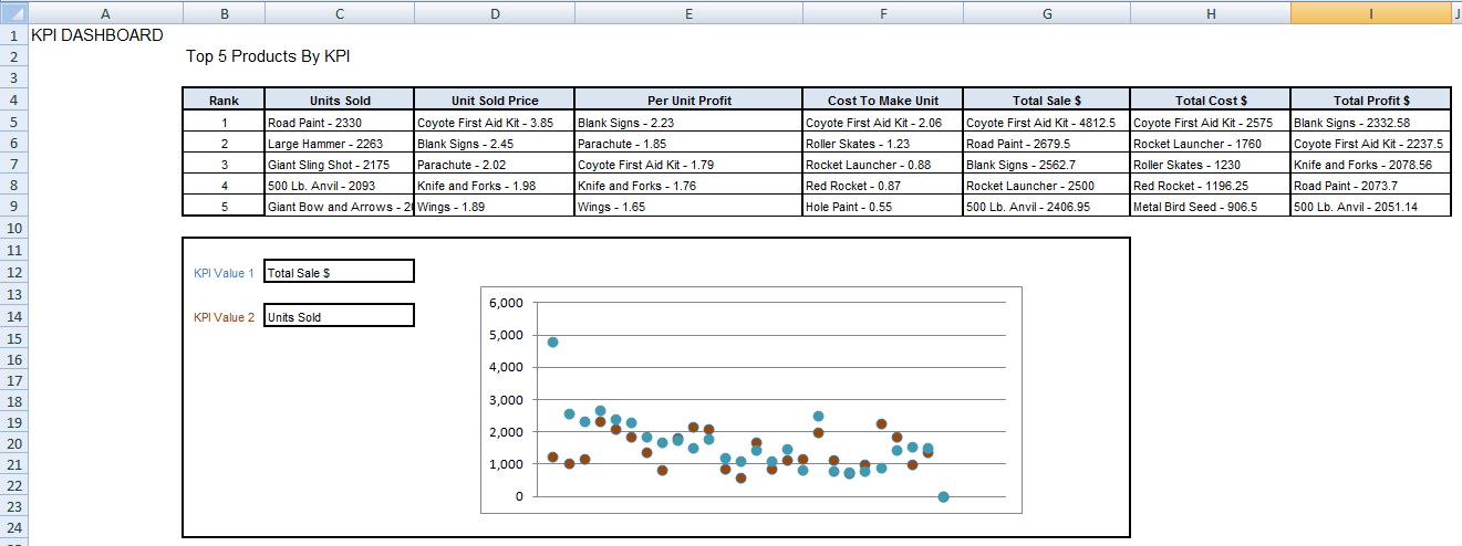
Now this is just a basic graph. I have not added target goals and projections. I only wanted to show how to create a basic KPI report. In another blog I will create a complete KPI dashboard with all the bells and whistles.
Subscribe to:
Posts (Atom)