Force Uppercase In Cell(s)

The other day my manager asked me an interesting question. He wanted to know if there was a way for force the contents of a cell to be all uppercase.

I thought for a minute and remember reading about how to do this. Well I could not remember where I learned of this trick but I did remember how to do it.

You can force the cell to have upper case using Data validation and the =Exact function.

From the menu select Data > Data Validation 

In the Settings tab enter =EXACT(B7,UPPER(B7)) in the formula field.

But we can jazz this up a bit. In the Input Message I can enter a message to display when the cell is selected.

For the Error Alert, I also create a message (since generic errors are sometimes confusing).

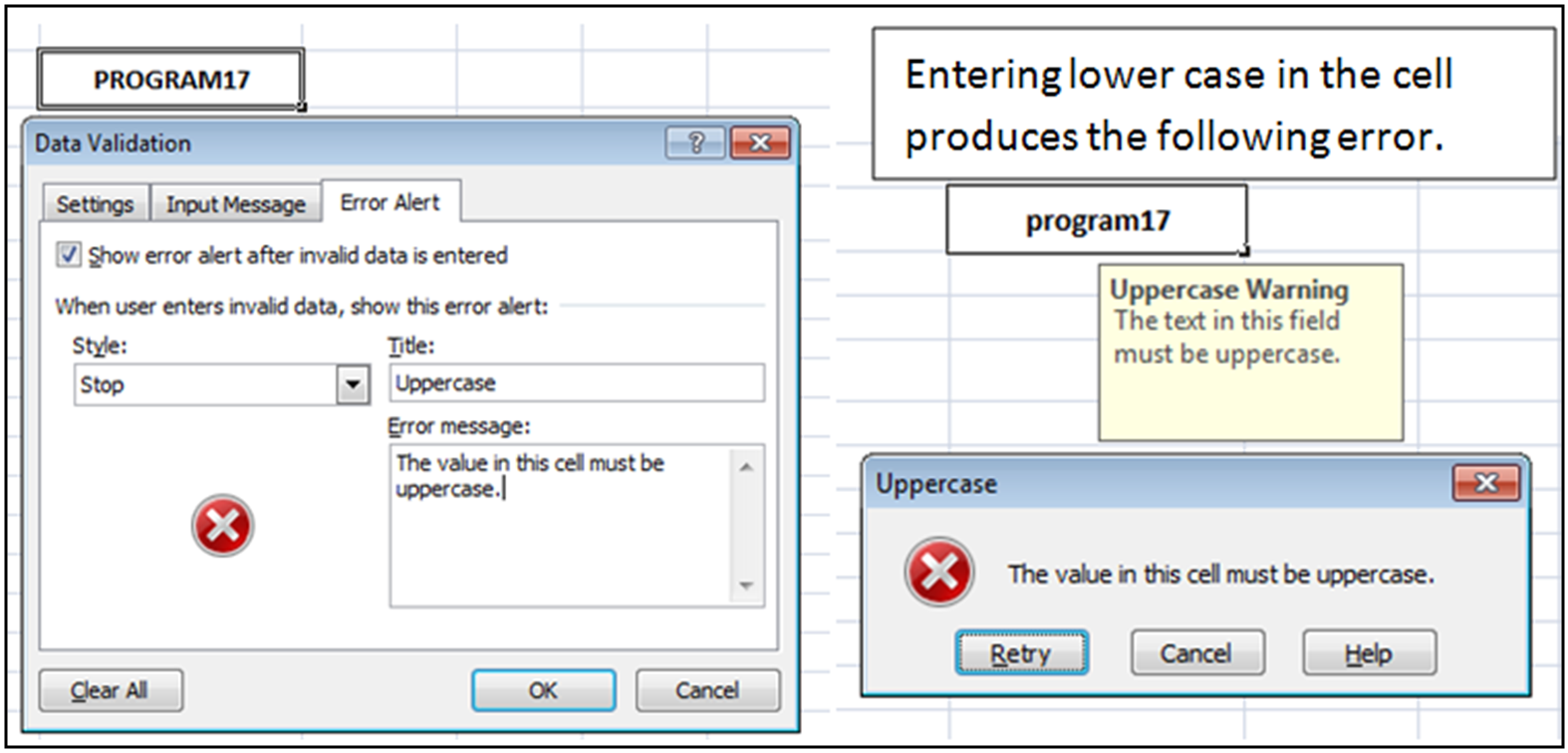
Now whenever someone selects the cell they get a prompt onscreen as to what type of data is expected and if they enter in the data incorrectly, they get an error message explaining how to correct the data.

So how does this work? Well Exact compares two values. In this case the Value in cell B7 compared against the Uppercase conversion of cell B7. The uppercase function converts the entire cell to uppercase.

So the next time someone asks you for ensure the values of a cell are uppercase, consider the above, break out your mad Excel skills, and WOW them.

INTERMEDIATE, EXACT, UPPERCASE, DATAVALIDATION

INDEX part 2

Last post I introduced the Index formula. In this post I want to continue explaining how Index works and why you should understand it.

From my previous post, we now know that Index allows you to get a value at an intersection of any give row and column. In this example I return the 4^th row down and the 3^rd column to the right for the data range.

Item	Price	Manufacturer		Result	Formula
Hammer	7.53	ACME West
Bird Seed	13.58	ACME East		ACME West	=INDEX(A2:C11,4,3)
Large Magnet	100.00	ACME South
Rocket Skates	68.54	ACME West
Safety Helmet	18.00	ACME North
Large Spring	240.00	Scotland
First Aid Kit	72.00	ACME East
Cannon Ball	45.00	ACME West
Rope	12.00	ACME North
Paint	22.50	ACME South

Now you can also return an entire row or column from the same table. Perhaps I want to know the total Price of all items in my table. I could write the formula =SUM(INDEX(A2:C11,,2)). And yes I know I could just Sum the column but this is an article on the Index formula. Our example formula ends ,,2 This tells the INDEX formula to return the entire column. If it ended in ,2, then Index would return the row.

Remember the syntax of INDEX. By omitting the Row Or Column reference I can return entire rows or columns.

=INDEX(Range,Row,Column)

Item	Price	Manufacturer		Result	Formula
Hammer	7.53	ACME West
Bird Seed	13.58	ACME East		599.15	=SUM(INDEX(A2:C11,,2))
Large Magnet	100.00	ACME South
Rocket Skates	68.54	ACME West
Safety Helmet	18.00	ACME North
Large Spring	240.00	Scotland
First Aid Kit	72.00	ACME East
Cannon Ball	45.00	ACME West
Rope	12.00	ACME North
Paint	22.50	ACME South

=INDEX’s unique ability to return entire rows or columns from ranges or arrays is very powerful.

Perhaps my dataset is large, spanning cells A2 thru AZ60000 (A2..AZ60000).  I can name that range LargeDataSet

I can then name individual columns in that dataset by referencing the Array. If I want to create another Name for the Index column (column 1) I would write the name formula as follows.

ITEM  =INDEX(LargeDataSet,,1)

This now allows me to lookup any item by using the =MATCH function.

Item	Price	Manufacturer		Result	Formula
Hammer	7.53	ACME West
Bird Seed	13.58	ACME East		5	=MATCH("Safety Helmet",Item)
Large Magnet	100.00	ACME South
Rocket Skates	68.54	ACME West		18.00	=OFFSET(A1,MATCH("Safety Helmet",Item,0),1)
Safety Helmet	18.00	ACME North
Large Spring	240.00	Scotland
First Aid Kit	72.00	ACME East
Cannon Ball	45.00	ACME West
Rope	12.00	ACME North
Paint	22.50	ACME South

In this example I use my name Range Item (A2..A30) to find the row Safety Helmet is on (row 5)

I then use Offset much like I would use Vlookup to return the price.

Using this method is comparable in speed to using Vlookup  when you are doing only 1 lookup. But I can look to the left with this method (Vlookup only looks to the right).

INDEX is useful in many other ways but that another future post.  Give INDEX a try and add it to your Excel knowledge.