VLOOKUP

+

Vlookup is one of the most useful functions available in Excel.

There are times that you will need to pull in data from different sections or tabs of a workbook (or even different workbooks).

Let’s say that you want to identify the Company Name for each of our Items in our sample workbook. VLookup will search for a value you provide in the left most column of a range of data and return the value in the same row based on an index number that represents the column where the data resides that you want to return. Confused???

Simply put, VLOOKUP allows you to search for an item and pull back related information to that item.

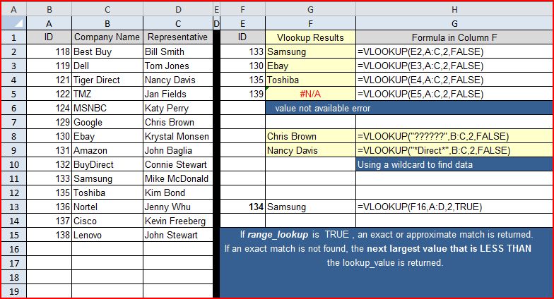
Take a look at our sample data. Columns A B and C has data about vendors. For my example I have also entered in the ID of some vendors in column E. I want to use VLOOKUP to return the Company name for each ID in column E.  I have entered in my VLOOKUP formula in column F. To see the formula, I have also typed the exact formula that I used in column F in Column G.

You will notice that in cell F5 I have a “value not available error”. This is because in cell E13 I have the value 134. That value is not included in my lookup range. (This can be corrected by using the IFERROR(VLOOKUP combination.)

If you compare one of my calculations in my sample workbook, you can see how each component works.

=VLOOKUP(E2,A:C,2,FALSE)

VLookup( value, table_array, index_number, not_exact_match )

Value: The value I want to search for (133).                                                                    

table_array: Is a selection of data that is at least two columns wide that is sorted in ascending order by the first column in the array (Columns A B and C).                                                                  

index_number: The column # in table_array where the data you want returned is stored in. Regardless of where you start your table_array, the first column is number 1. (2 – Return Column B)                         

Not_exact_match: True or False option. Enter False to return an exact match. Enter TRUE to find an approximate match. If no exact match is found, True will look for the next largest value that is less than value 

(False – find an exact match).

Wildcards

If range_lookup is FALSE and lookup_value is text, you can use the wildcard characters - (?) and asterisk (*).

A question mark matches any single character (as shown in cell F8 in my example).

 If you have 6 question marks, then you are trying to return a field with 6 characters in length.

An asterisk matches any sequence of characters.

 If you want to find an actual question mark or asterisk, type a tilde (~) preceding the character.

VLOOKUP also has a cousin called HLOOKUP but that’s a topic for another time.

How have you used VLOOKUP to solve a problem?