
There are times when we want to call attention to key items in data. Perhaps it’s a change in profit or drop in inventory. Keeping the data all in one color can cause someone to overlook the key point of a report.
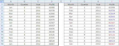
Fortunately Excel allows us to use Conditional Formatting to resolve this problem. In this example I have the same data displayed two ways. I have highlighted the Profit column in the second version to indicate if the value has gone up, down or remained the same.

By using Conditional Formatting on only the one column of data, I point out the most important part of the report and provide the reader a quick visual way to see how the data is trending (without having to manually compare each value to identify the trend).
To create this report, I start with my first chart then use formulas to reproduce it.

Yes I know that I could just apply the conditional formatting to my original data but that would spoil the cool bling bling technique that I will apply later on in this lesson.I want to start my conditional formatting on the second row of data as the first row does not have any reference to prior value. I select Cell I3 and then Create a New Conditional Formatting Rule
Home > Conditional Formatting > New Rule > Use a formula to determine which cells for format.

The formula I want to enter is =D2<D3. I want to select the format button and select a blue color for the font. Now whenever the current cell is greater than the previous cell, the font will be blue.
I repeat the process with a red font
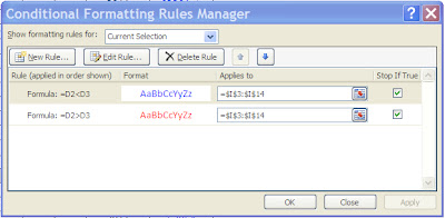
When done, I have two rules….
Next I just copy I3 down to all the other cells in column I for the remaining months.
This image is of the Conditional Formatting Rules Manager after I have copied the formatting into the rest of the other cells.
Try replacing the formula in cell I3 with the following…

Please, keep your applause down to a minimum……
What this formula does if append the value of D3 with either and up arrow, down arrow or dot.
=D3 & " " & IF(D2<D3,"▲", IF(D2=D3,"●","▼"))
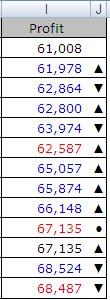
If you can do that, then you could also change the arrows to match the color of the numbers
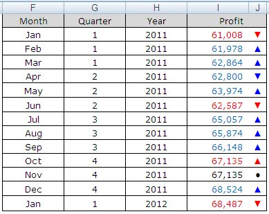
Lastly my favorite, black text for the numbers with blue and red indicators in the helper column. I have created the boarders so it appears to be in the same cell.

Break out this technique at the next quarterly review and watch everyone’s face as they try to figure out how you did this.

By using Conditional Formatting on only the one column of data, I point out the most important part of the report and provide the reader a quick visual way to see how the data is trending (without having to manually compare each value to identify the trend).
To create this report, I start with my first chart then use formulas to reproduce it.

Yes I know that I could just apply the conditional formatting to my original data but that would spoil the cool bling bling technique that I will apply later on in this lesson.
Home > Conditional Formatting > New Rule > Use a formula to determine which cells for format.

The formula I want to enter is =D2<D3. I want to select the format button and select a blue color for the font. Now whenever the current cell is greater than the previous cell, the font will be blue.
I repeat the process with a red font
but make the formula =D2>D3.
When done, I have two rules….
Next I just copy I3 down to all the other cells in column I for the remaining months.
This image is of the Conditional Formatting Rules Manager after I have copied the formatting into the rest of the other cells.

Now your spreadsheet is Da Bomb…. Or is it???

Try replacing the formula in cell I3 with the following…
=D3 & " " & IF(D2<D3,"▲", IF(D2=D3,"●","▼"))
Now copy it down to the other cells below.
Please, keep your applause down to a minimum……
What this formula does if append the value of D3 with either and up arrow, down arrow or dot.
=D3 & " " & IF(D2<D3,"▲", IF(D2=D3,"●","▼"))
That’s why I could not just apply the conditional formatting to my original data at the beginning of this lesson. I wanted to be able to add the indicators to my value.
Getting the indicators takes a bit of fore thought. When you want to create this formula from scratch, do it in MS Word and you can find the indicator when you insert a symbol. Once you have the formula written, copy it back to Excel.
How about breaking out the indicators into the adjacent column and then you could format the Profit column with an Accounting Number format?

If you can do that, then you could also change the arrows to match the color of the numbers

Lastly my favorite, black text for the numbers with blue and red indicators in the helper column. I have created the boarders so it appears to be in the same cell.

Break out this technique at the next quarterly review and watch everyone’s face as they try to figure out how you did this.
No comments:
Post a Comment