Filtering Data in Excel - Become awesome at understanding your data

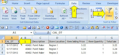
This week I would like to focus on Excel filters. Filters allow you to analyze and break down large amounts of data on a spreadsheet. Perhaps you have a large list of sales broken out by date of sale and store location. It would be useful to be able to slice this data up so that I could see sales on a specific day for a specific location. Sorting is not the best way to view this since I may want to view Region 3 and that would be in the middle of my data. Here is where filtering shines.

Setting the filter is easy as 1,2,3. Start by selecting the row or header cells you’d like to filter, select the “Data” tab at the top of the screen. Then click “Filter”.

Now select the column you want to filter and click on the downward arrow (I choose Cal_Dt). This will display a grouped list of all the items in that column. If the column contains a date field, then the data filter will allow you to select an entire year, month or individual days. If you only want to select one day, uncheck the (Select All) option then choose the day(s) you want to view.

In this example I only want to look at Sales for May 20th. So I uncheck the (Select All) option then check only the May 20th box. When you do this you will notice that the Month and Year box shades dark. This indicates that you have selected a subset of data in the list. When I am done I click on the OK button.

Now my data is filtered. You will notice that displayed filtered rows are highlighted blue and the rows that do not have May 20^th as the date are now hidden.  The lower left hand corner of Excel will also display a list of records that are found.

“Ready    26 of 99 records found”

I can repeat this process filtering on Region 3. When I click on Store Location only results that are in my already filtered 5/20/2012 date are displayed (a subset of Store Location). Now I can see the Sales for 5/20/2012 for Region 3. Notice that rows 66 and 77 are displayed. Rows 67 through 76 do not meet the requirement of the selected date and Store Location and therefore are hidden.

Columns that are filtered have a funnel shape instead of a drop down arrow. This provides you with a visual clue as to what columns you have applied a filter to.

It’s also important to mention that you can filter by other options. If you remember the original date filter, you could have also selected an option called “Date Filters” (since this is a date field). This will provide you with a variety of other options that you can choose.

It you are filtering on a number field the “Number Filters” would show the following…

And a text field would have a “Text Filters” and would show…

With the newer versions of Excel you can even filter on color.

In this example I have some highlighted fields…

When I click the drop down arrow in the Description column I get the option to filter by color…

To remove a filter I can click on a single column that has a filter applied and choose the clear filter from option. To remove all filters from your data you can return to the Ribbon and uncheck the Filter option on the Data Tab.